Resort Rooms & Suites
Start Planning
Let our experienced team at Hawks Cay Resort transform your vision into a flawless weddings. Contact us today to begin planning your perfect weddings or event.
Let our experienced team at Hawks Cay Resort transform your vision into a flawless weddings. Contact us today to begin planning your perfect weddings or event.